A simple ODE Solver Using Python

In this blog post we will understand what is an ODE and how to solve it numerically using Python.

What is an ODE?

In mathematics, an ordinary differential equation (ODE) is a differential equation containing one or more functions of one independent variable and the derivatives of those functions ¹ .

Why do we need numerical methods?

Numerical methods are techniques to approximate mathematical procedures. Here we are approximate an time integral. We use numerical methods when an analytical solution does not exist (e.g. Navier Stokes Equations), or an analytical method is intractable.

Fundamental Approach: Euler’s Method

Here we want to solve an ODE in the form of

\[\frac{dx}{dt} = f(x,t)\]

Using Taylor series expansion around \(x(t_0)\) we can write following equation

\[x(t_0+dt) = x(t_0) + dt \cdot x'(t_0) + O(dt^2)\]

This method is called (Explicit) Euler’s method.

Physical Problem

Let’s consider the falling of a parachute jumper. Governing equation for this problem is \(F=m*a\) . To model the drag force we choose simple model \(F_{drag}=\frac{1}{2}\rho A C_D V^2\), where \(C_D\) is drag coefficent, \(A\) is area of parachute and \(\rho\) is air density. The other forces acting on the jumper is gravitationa force which is given by \(F_G=g*m\), where \(g\) is gravitational acceleration and \(m\) is mass. Resulting governing equation is the this problem is:

\[m \cdot g - \frac{1}{2}\rho A C_D V^2 = m \cdot a\] \[a = g- \frac{\rho A C_D V^2}{2m}\]

In other words,

\[\frac{dV}{dt} = g- \frac{\rho A C_D V^2}{2m}\]

Let’s code it

First of all we need to import libraries to python. In this project we will use 2 libraries called numpy and matplotlib.

import numpy as np
import matplotlib as plt

After importing libraries we will define the ODE’s function

def dvdt(V,t):
    a = g- rho * A * cd * V**2 / 2 / m
    return a

Since this is a rather simple ODE we have an analytical solution, which we will be use to check accuracy of solution.

def analyticalsol(t):
    v = (21.0262 * np.exp(0.933124 * t) -21.0262) / (np.exp(0.933124 * t) + 1)
    return v

This gives us the derivation of function at the a known point.

Let’s initialize the variables

v_0 = 0       #m/s    initial velocity
t_0 = 0       #s      initial time
t_end = 10  #s      end time
m = 100     #kg     mass
A = 3.14    #m^2    area
cd = 1.15   #       drag coefficent
rho = 1.229 #kg/m^3 air density
g = 9.81    # m/s^2 gravitational acceleration
dt = 1      #s      timestep

result = []  #empty of numerical results
time = []    #empy list of numerical time series

Now lets write the main solution loop

v=v_0  #Initialize Velocity
t=t_0  #Initialize Time
while (t < t_end):
  time.append(t)            #Store Current Time
  result.append(v)          #Store Current Velocity
  acceleration = dvdt(v,t)  #Get Acceleration
  v += acceleration * dt    #Advance velocity
  t += dt                   #Advance time

a_time = numpy.linspace(t_0,t_end,num=50) #Sample 50 Point betwen t_0 and t_end
a_result = analyticalsol(a_time)                #Get the solution

#Plot Analytical Solution
plt.plot(a_time, a_result, label="Analytical Solution")
#Plot Numerical Solution
plt.plot(time, result, label="Numerical Solution")
plt.legend()  #Add Legend
plt.grid()    #Add Grid
plt.show()    #Show plot on the screen

You can download the python script that I used to produce result below from here.

Results

Comparision of Solution.

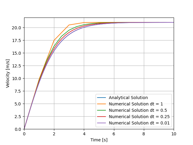
Here we can clearly see that as we decrease the timestep we get a more accurate solution. There is a limit we can decrease the timestep, while decreasing we error. Using too small or too big timesteps causes inaccurate results.

1. Dennis G. Zill . A First Course in Differential Equations with Modeling Applications. ↩